- Published on
Intro Computer Vision topics - CPSC 425 (UBC)
- Authors

- Name
- Christina Yang
This is a compilation of my main takeaways from CPSC 425 (2023W). Information source: The University of British Columbia
Disclaimer: This is not a reliable source of information. May contain mistakes.
Table of Contents
- What is Computer Vision?
- Problems with Computer Vision?
- Image formation
- Image Filtering
- Sampling
- Template Matching
- Scaled Representations
- Edge Detection
- Corner Detection
- Texture
- Local Image Features
- Planar Transformations
- Stereo
What is Computer Vision?
- Inverse of Computer Graphics
- Graphics creates images, vision parses/understands images
- Let computers see like humans
- Label objects in image with neural networks
- Face detection with template matching
- We often know what should go in images with gaps. Computers can fill the blanks with texture
- See multiple images of a scene, and piece together the images for a wholistic view with Panorama stitching
Problems with Computer Vision
- 3D->2D
- Real life is so much more complex
- Cannot invert image formation process
- Human vision -> computer vision
- we have LOTS of neurons working on this tasks, doing the same with a computer is computationally expensive
- We don't fully understand how our own vision works
- Search through visual data
- Lots going on in an image, scale is enormous
- Algorithms for manipulation or creation of image or video content (visual imagination)
- Have to deal with wonky lighting, different scales, items in images being deformed, context, motion, blending in with background, blurring, same types of items (ex. chair) looking very different from each other, etc.
Image Formation
Light - Reflectance - Cameras and Lenses
Pinhole
- Most basic camera type.
- Viewing through a smaller hole can make image sharper.
- If the hole is too big, won't be too sharp, since light from too many directions
- If hole is too small, diffraction increases, which also causes blurring due to how light waves interfere with each other.
- Very slow, not a lot of light goes through at a time
- Dark, hole is too small, not a lot of light goes through
The pinhole, often no larger than the head of a pin (hence the name), serves as a gateway for light rays. As these rays travel through the pinhole, they create an inverted image on the opposite side of the box. Unlike conventional cameras with complex lenses, the pinhole camera relies solely on the principles of light and the art of geometry.
The pinhole camera, in its simplicity, reveals the fundamental nature of light and image formation. Changing the size of the pinhole alters the sharpness and brightness of the resulting image. The distance between the pinhole and the imaging surface affects the focus.
(source: ChatGPT, edited by me)
Real lens
Real cameras must have a specified aperture (hole) size. They are complex with multiple stages and elements to deal with issues such as blurring, chromatic aberration (different colours bent by different amounts), vignetting (light fall off at image edge) and sharp imaging across the zoom range. Lenses overcome limitations of the pinhole model while trying to preserve it as a useful abstraction
Projection equations: perspective, weak perspective, orthographic
Project 3D point to 2D. Weak perspective (including orthographic) has simpler mathematics — accurate when object is small and/or distant — useful for recognition Perspective is more accurate for real scenes TODO: add info about orthographic projection
Image Filtering
Image as a function, Image Transformations, Linear filters, Correlation and Convolution Gaussian, Pillbox filter, Separability, Low Pass / High Pass Filtering
| Filter | calculations | properties | linear | low-pass | use |
|---|---|---|---|---|---|
| Box (avg) | - separable - doesn’t model lens defocus well | Y | Y | ||
| Gaussian | - separable - rotationally invariant | Y | Y | - smoothing, resizing | |
| Pillbox | - not separable - rotationally invariant | Y | Y | - a better model for defocus | |
| Median | N | - Effective at reducing certain kinds of noise, such as impulse noise (a.k.a ‘salt and pepper’ noise or ’shot’ noise) | |||
| Bilateral | - edge preserving | N | - denoising - cartooning - flash photography | ||
| ReLu | Negative numbers become zero | - output size = input size | N |
Low-pass filter: filters out all of the high frequency content of the image, only low frequencies remain
Linear properties (I=image):
- superposition (F
1+F2)I=(F1I+F2I) - scaling
- shift invariance
Dealing with boundaries:
- pad with zeros
- ignore (results in smaller output)
- wrap (use top row as most bottom, left as right) like a circle or teleportation portal
Speed up convolution using:
- separable filters
- For n x n pixels and m x m multiplications
- Separable means O(2m+n^2^) instead of O(m^2^+n^2^)
- Fourier Transforms if the filter and image are both large
Characterization Theorem: Any linear, shift invariant operation can be expressed as convolution Correlation: X + i, Y + j Convolution: X - i, Y - j, (Correlation rotated by 180 deg) ex. 9a + 8b + 7c + 6d + 5e + 4f + 3g + 2h + 1i
Equations to memorize: Gaussian

Applications of image filtering
- Used in CNNs
Sampling
Sampling Theory, Bandlimited Signal, Nyquist Rate, Aliasing, Color Filter Arrays, Demosaicing, Digital Imaging Pipeline
Why sample?
We sample to reduce size or amount of space used.
If we aren't careful with sampling, we can end up with an image or audio clip with weird distortions (aliasing) in areas with high frequencies. Because of this, it is a good idea to use a low-pass filter to remove high frequencies before sampling, or just sample more.
Well how can we know which high frequencies to remove?
Turns out we can avoid aliasing if we sample at over twice the maximum frequency (Nyquist Sampling Theorem). Note that this also means that the image or audio clip must HAVE a maximum frequency (=is bandlimited).
Bandlimiting in images is limiting the maximum spatial frequency.
What exactly is aliasing?
High frequency in this context means more changes in a small interval.
Small details are examples of high frequency elements, while a long expanse of just blue sky would have a low frequency.
The problem with small details is that when you remove part of it, the rest looks (or sounds) weird. This isn't a problem with low frequency items, since if you remove a speck of blue sky, well the rest is still blue sky so you can't tell the difference.
Ever wondering how cameras reconstruct images?
Answer: Demosaicing
Lots of digital cameras use color filters to differentiate colors. The problem is that each pixel can only store information about one color channel (red, green, or blue). Because of this, lots of color information will be missing. Demosaicing is the process of reconstructing the full image from the incomplete information.
One method of demosaicing is Bilinear Interpolation. This involves averaging your 4 neighbours for each color channel.
Which four neighbours to use depends on what works best for that channel (with how it is spaced out). Options include: your directly touching neighbours (up down left right) or your 4 diagonal (corner) neighbours.
For red and blue (regular grid with 2 pixel spacing): 1/4 * [1 2 1 2 4 2 1 2 1]
Bilinear Interpolation doesn't work that well in practice, there are more complex methods that do the same thing, taking edge information into account.
White balance
We perceive different illuminances as white, and this illuminance depends on the environment. Because of this, when the environment is removed or changed, we need to adjust the illuminance accordingly, so it doesn't look too strong.
Exponential relationship between human perceived brightness and luminance. "Equal steps in human perceived brightness are achieved by increasingly large steps in luminance (sensor counts)" - Source (couldn't phrase it better)
Storing bits we can't really tell apart is wasteful, so instead we store use gamma corrected encoding (V).
Not sure where this is relevant, but we see mid-frequencies better than low and high frequencies.
Template Matching
Template Matching, Correlation, Normalised Correlation, SSD
Find a template in an image.
We need some mathematical way of telling whether the image patch is similar to the template.
- images can be represented as matrices of rgb values,
correlation= dot-product (element-wise multiply then sum) of the template and a patch of the imagecorrelationis higher when there is more correlation
correlationis also higher due to greater brightness, so we need to normalizecorrelation.- divide by magnitude of template and magnitude of image patch
- normalized correlation between -1 and 1, 1 means identical
- some correlation
thresholdin order to indicate a match. - Repeat correlation calculations (steps 2-4) for each possible alignment of template and image
Note: another method is to minimize SSD between image patch and template (I-J)^2^ instead of maximize normalized correlation (NCC). NCC is less sensitive to brightness and contrast.
Common causes of failure
— Different scales — Different orientation — Lighting conditions — Left vs. Right hand — Partially hidden — Different Perspective — Motion / blur
In 3D:
- viewing direction and pose
- conditions of illumination
We like template matching/linear filtering due to the easy computations, and working well with noise, but there's a lot of downsides.
Scaled Representations
Gaussian Pyramid, Laplacian Pyramid, Pyramid Blending, Multi-Scale Template Matching and Detection
We can address different scales in template matching by creating multiple versions of the image in different sizes, and attempting to match in each one. Different sizes also lets us look for different levels of detail/blurring/spatial frequencies.
Previously we talking about low-pass filtering first before sampling to reduce size. We use this method here to construct the image in different scales.
Gaussian pyramid is one method on constructing the different scales. We first gaussian blur, then reduce size. We repeat this process of blurring, then reducing size, to get a pyramid of images at different scales and blurriness.
Laplacian Pyramid is what was removed from the original image after gaussian blurring. Storing this allows us to reconstruct the original image. It also is a band-pass filter.
Pyramid/image blending
Use laplacian to preserve details, and use gaussian to blend different images together.
- Build Laplacian pyramid LA and LB from images A and B
- Build a Gaussian pyramid GR from mask image R (the mask defines which image pixels should be coming from A or B)
- From a combined (blended) Laplacian pyramid LS, using nodes of GR as weights: LS(i,j) = GR(i,j) * LA(i,j) + (1-GR(i,j)) * LB(i,j)
- Reconstruct the final blended image from LS Source
Edge Detection
Image Derivatives, Edge Filtering, 2D Gradient, Canny Edge Detection, Image Boundaries
What is gradient in an image? The gradient points in the direction of most rapid increase of intensity
Use derivatives to find edges. Calculate derivative in X and derivative in Y. Just seeing the derivatives is usually not enough, due to noise. So we first smooth, then calculate derivatives.
Derivative approximations: Central: [-1 0 1] Forward: [-1 1] Backward: [1 -1].T
The goal of the first filter is to calculate the central difference, so if you were to convolve the first filter with the image to get this difference, you would actually convolve the image with [1, 0, -1]. Source: TA Not sure what this means. Do we use [-1 0 1] or [1 0 -1]?
Sobel Edge Detector:
- calculate derivative using central differencing
- edge if pass threshold
Canny Edge Detector local extrema of a first derivative operator Uses two threshold. A strong threshold, and a weaker one for if it connected to an edge.
- Apply directional derivatives of Gaussian
- Compute gradient magnitude and gradient direction
- Non-maximum suppression — thin multi-pixel wide “ridges” down to single pixel width
- Linking and thresholding — Low, high edge-strength thresholds — Accept all edges over low threshold that are connected to edge over high threshold Source
Corner Detection
Image Structure, Corner Detection, Autocorrelation, Harris, Scale Selection, DoG
Texture
Texture Representation, Filter Banks, Textons, Non-Parameteric, Texture Synthesis
Local Image Features
Correspondence, Invariance, Geoemtric, Photometric, SIFT, Object Instance Recognition
Say we want to match features in two different photos. We need a method that can account for scaling, rotation, etc. (aka a more robust method than template matching)
SIFT (Scale Invariant Feature Transformation) Descriptor
Construct gradient histogram
- Describe local region by distribution (over angle) of gradients
Detector: find points that are maxima in a DOG (Laplacian of Gaussian) pyramid Descriptor:
- Take local gradients in these points. Create a histogram out of their angles/orientations.
- Histogram has 8 orientations, 4x4 grid -> Each SIFT feature is represented by 8x4x4=128 numbers
- this makes your descriptor invariant to scale/orientation
- Normalise the final descriptor to reduce the effects of illumination change Match Ratio Test:
- Compare ratio of distance of nearest neighbour (1NN) to second nearest (2NN) neighbour — this will be a non-matching point
- Rule of thumb: d(1NN) < 0.8 * d(2NN) for good match
- Greater distances means we are more confident that the 1NN is the correct match Problem:
- Repetitive structures means multiple matches, how do we know which one is right? Solution: RANSAC
Planar Transformations
2D Transformations, Similarity, Euclidan, Affine, Homography, Robust Estimation, RANSAC
Panoramas (merging images together)
Images can come in different orientations + scales + shears. Sometimes, we need to apply a linear transformation to put the images in the same orientation/scale/shear.
Similarity transform is the most simple kind. I believe it is just translation and rotation, and it preserves orientation.
Affine is one kind of linear transformation that preserves parallel lines.
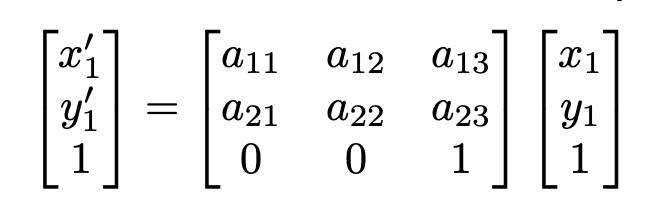
Affine: multiply coordinates by a weight, then add bias, which can be represented as a single matrix:

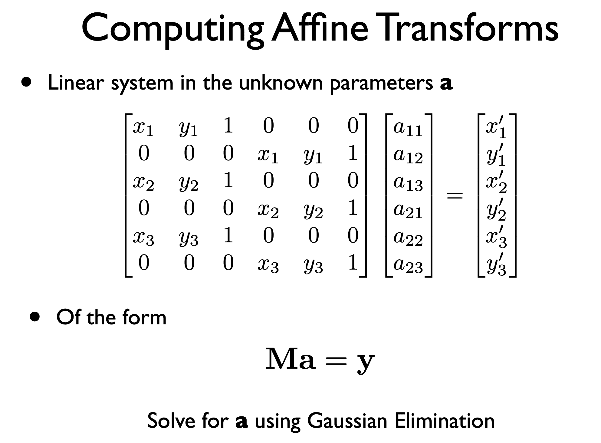
How can we know what affine transformation to apply? We need to find the affine matrix to multiply by.

- We have the matching coordinates in both images, so we can solve for the affine matrix.
- Use matrix to transform image.
Another transformation we use is projective (homography). This is more flexible than affine, since it does not preserve parallel lines – it only preserves straight lines.

Since projective transformations involve more unknowns, we use SVD to calculate the matrix.
Since there are many matching points, we will get many different transformation matrices. How do we know which one to use? Enter RANSAC:
RANSAC
- Match feature points between 2 views
- Select minimal subset of matches
- Similarity transform requires at least 2 corresponding points from source and destination images to get transformation matrix
- Affine = 3 points, Homography = 4 points
- using minimal subset is more robust to outliers + fewer calculations/faster to compute
- Compute transformation T using minimal subset
- Check consistency of all points with T — compute projected position and count #inliers with distance < threshold
- Repeat steps 2-4 to maximise #inliers
RANSAC is needed, because just features matching results in many outliers. RANSAC finds us a subset of matches that all agree on an object and geometric transform (e.g., affine transform). We like RANSAC because it is easy to implement, and easy to estimate/control failure rate
How many samples should we use for RANSAC? We need a 0.99% probability of one good sample.
Stereo
Epipolar Geometry, Rectification, Disparity, Block Matching, Occlusions, Ordering Constraints
What about rotations in 3D? Linear transformations cannot deal with 3D transformations. Instead, we use Epipolar geometry for this.
We transform (rotate) images so that their epipolar lines are horizontal.
This is necessary in stereo matching, since stereo matching involves multiple cameras.
- Rectify images (make epipolar lines horizontal)
- For each pixel in image 1 a. Search along epipolar line in image 2 b. Find best match and record offset = disparity c. Compute depth from disparity
- With two eyes, we acquire images of the world from slightly different viewpoints
- We perceive depth based on differences in the relative position of points in the left image and in the right image
- Stereo algorithms work by finding matches between points along corresponding lines in a second image, known as epipolar lines.
- A point in one image projects to an epipolar line in a second image
- In an axis-aligned / rectified stereo setup, matches are found along horizontal scanlines
Optical Flow
Brightness Constancy, Optical Flow Constraint, Aperture Problem, Lucas-Kanade, Horn-Schunck
How do we deal with motion in images? How do we match two images at different time-steps? Assuming image intensity does not change as a consequence of motion, we obtain the (classic) optical flow constraint equation: Ixu + Iyv + It = 0 [u, v] are motion, Ix, Iy, It are partial derivatives
Lucas–Kanade is a dense method to compute the motion, at every location in an image
Aperture problem: We don't know which way the object is actually going, especially if part of it is hidden.
Multiview Reconstruction
Multiview Matching, Bundle Adjustment, Pose Estimation, Triangulation, Image Alignment and 3D Reconstruction
Panoramas pt.2
Panoramas need to account for motion + 3D rotation stuff, so what we did previously with 2D image stitches isn't enough.
- Match features, e.g., SIFT, between all views
- Use RANSAC to reject outliers and estimate Epipolar Geometry / Camera matrices
- Form feature tracks by linking multiview matches
- Select an initialization set, e.g., 3 images with lots of matches and good baseline (parallax)
- Jointly optimize cameras R, t and structure X for this set
- Repeat for each camera:
- Estimate pose R, t by minimising projection errors with existing X
- Add 3D points corresponding to the new view and optimize
- Bundle adjust optimizing over all cameras and structure
Visual Classification
Instance and Category Recognition, Viusal Words, Bag of Words, Support Vector Machines Linear Classification, Nearest Neighbour, Nearest Mean, Bayesian Classifiers, One-Hot Regression, Regularisation, SGD, Momentum
What if we want to use RANSAC to label images? Can we?
RANSAC will work, except it fails with large appearance variation (intra-class variation). For example, if you want to label an object as an owl, well there are many species of owls and they look very different from each other.
Instead, we will need a collection of local features (bag-of-features) that correspond to that object. bag-of-features: • deals well with occlusion • scale invariant • rotation invariant
- we quantise feature descriptors
- use k-means to cluster similar features together
Bag-of-words (BOW) Dictionary Learning: Learn Visual Words using clustering Encode: build Bags-of-Words (BOW) vectors for each image Classify: Train and test data using BOWs
Construct Visual Dictionary
Compute Histogram of Visual Words
Initialize an empty K -bin histogram, where K is the number of codewords
Extract local descriptors (e.g. SIFT) from the image
For each local descriptor x
- Map (Quantize) x to its closest codeword → c(x)
- Increment the histogram bin for c(x)
Return histogram We can then classify the histogram using a trained classifier, e.g. a support vector machine or k-Nearest Neighbor classifier
Neural Networks
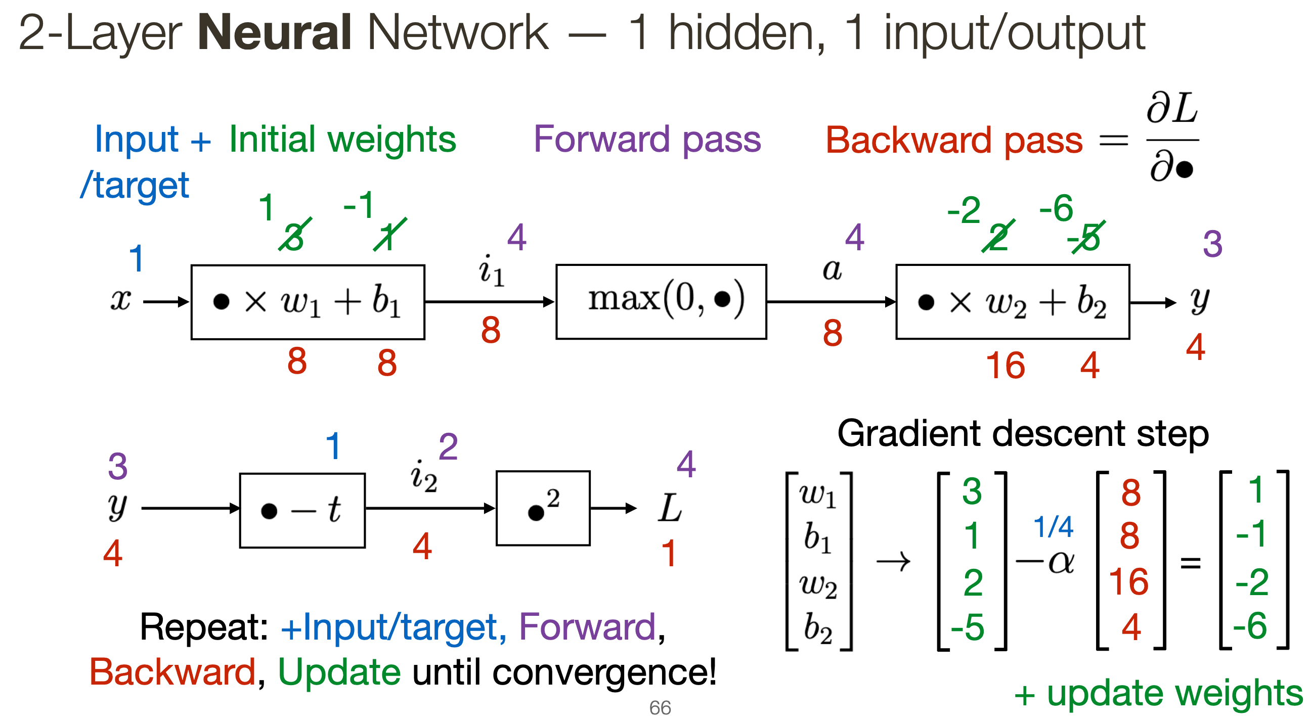
Activation Functions, Softmax, Cross Entropy, Update rules, Perceptron, 2-layer Net, Gradients, Backpropagation Linear layer backward pass, Convolutional Neural Networks, Strided convolution, Max Pooling, Deep Learning, AlexNet, VGG
- Basic operations in CNNs are convolutions (with learned linear filters) followed by non-linear functions.
- A convolutional layer applies a set of learnable filters
- A pooling layer performs spatial downsampling

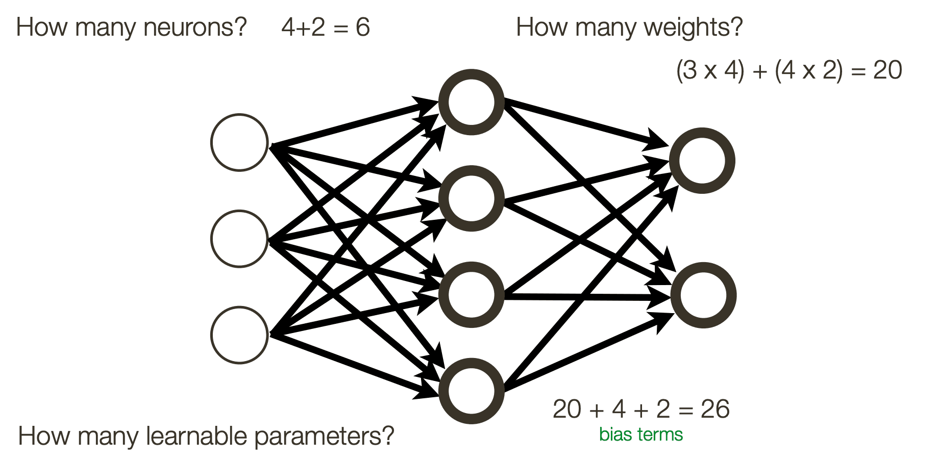
Neurons: number of nodes excluding inputs (includes outputs) Weights: arrows connecting nodes

Layers
- More layers = more complex functional mapping
- More efficient due to distributed representation
Perceptrons + linear + softmax regressors are limited to data that are linearly separable
Activation functions: Sigmoid, ReLu
Applications of Neural Networks
Make computers see what we see. Label objects in photo with what the object is.
Colour
Cone responses, Colour matching, Colour Spaces, RGB, XYZ, LAB, HSV, YCbCr Humans have trichromatic vision. We only perceive red, blue, and green, these are monochromatic. RGB is good approximation, some colors can only be matched subtractively
HSV: Hue, Saturation, Value Useful for colour selection applications, since it is a humanly natural way of describing color.